Introduction

Background and Rationale for this Study

According to Plant, lower middle economies (excluding India, China, and Venezuela) as of end-2019 had SDR allocations to the tune of US$18.73 billion, and the proposed allocations stand roughly at US$58.28 billion. But to achieve SDR allocation targets of up to 10% of GDP, these economies need US$429 billion. The achievement of such SDR allocations will have significant implications for exchange rate volatility. Hence, to overcome such exchange-related risks, a better solution was explained by Plant (n.d.), where high-income countries freely share their part of the SDR with lower-middle-income countries. For all practical purposes, this is better but not an easy solution.

To research this topic, Gagnon (2020) from the Peterson Institute of International Economics suggested that, in the wake of the COVID crisis, developed economies with strong and less volatile currencies must support depreciating and highly volatile currencies. Lower middle-income economies have experienced higher volatility and a significant decline in exchange rates as a result of reduced exports (external supply shocks) and portfolio withdrawals. The article spoke about G20 nations and in particular about the instability in energy exports.

In the same vein, the Trade and Development Update report from UNITAD (Mar 2020) highlighted that developing economies, unlike developed economies (which are facing a high consumer debt burden due to ‘easy’ and speculative debt availability), have issues with much dependability on exports (for which imports are also required) and the sale of their reserves. At the beginning of the crisis, as mentioned in the report (from late February to March 2020), almost ‘double’, that is, roughly US$59 billion, in foreign portfolio outflows (debt and equity combined) were witnessed compared to that in the era of the 2008 crisis. The biggest worry is the increased exposure to foreign capital in the form of debt in these emerging economies. Addison et al. (2020) added that stronger global supply chains had resulted in much higher spillover effects from both internal and external demand shocks. Baldwin (2020) rightly explained the concept of ‘shield packages’ compared to stimulus packages, since in COVID-19, with or without robust health measures, the recessionary downturn can be averted (although the recovery may be slow but certain).

Table 1. Unit Root Test* (ADF-GLS test).

Note: *The figures depict the p values and are based on the first differences of logarithmic conditional export volatility (every month). All p values are considering the rejection of unit roots (However, as a state of caution, it is advised to restrict the use of excessive differencing since in certain studies unit roots cannot be avoided). As mentioned in the text, here first differences of logarithmic conditional volatility of import, International liquidity and SDR exchange rates also followed the unit root tests and their p values also reflected the <0.05 level characteristics. Hence, only export volatility series unit root tests are exhibited as an indication.

The Yale Program in Financial Stability (YPFS), investigated lower-middle-income economies in terms of interest rate management and other relevant macroeconomic measures. Further, Purohit (2020) described how India spends nearly 0.8% of its GDP on the COVID crisis, compared to double-digit percentages of GDP as the stimulus in the USA, Europe, and China. Second, the liquidity measures through the monetary route had yet to witness their benefits in terms of boosting the supply crisis. From the Indian context, measures announced by the RBI in August 2020 to reduce systemic risks, including a temporary relaxation on SLR securities or special open market operations, have seen a mixed response.

How was the Emerging Economies Doing in the Pre-COVID Era or After the 2008 Global Meltdown?

How were the emerging economies doing in the pre-COVID era or after the 2008 global meltdown?

It is important for any macroeconomic study to provide relevant facts to justify the need and purpose. Tables 2–5, corresponding to the exchange rates, show the actual average values of exports, imports, international liquidity (in millions of dollars), and SDR reserves (in millions of dollars). These four economic variables were analysed with their respective growth rates across the two phases, that is, the early-COVID phase and the mid-COVID phase.

 Table  2. Monthly Export Figures of LMI South Asian Economies (Figures in $M scaled).

Notes: *Average early-COVID period (i.e., April 2013 till November 2019 monthly export data).

**Average during-COVID period (i.e., December 2019 till June 2020 monthly export data).

 Table  3. Monthly Import Figures of LMI South Asian Economies (Figures in $M scaled).

Notes: *Average early-COVID period (i.e., April 2013 till November 2019 monthly import data).

**Average during-COVID period (i.e., December 2019 till June 2020 monthly import data).

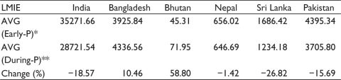
Table 4. Monthly International Liquidity Figures of LMI South Asian Economies (Figures in $M).

Notes: *Average early-COVID period (i.e., April 2013 till November 2019 monthly international liquidity data).

**Average during-COVID period (i.e., December 2019 till June 2020 monthly international liquidity data).

Table 5. Monthly SDR-Exchange Rates Figures of LMI South Asian Economies (Figures in $M).

Notes: *Average early-COVID period (i.e., April 2013 till November 2019 monthly SDR-Exchange rates data).

**Average during-COVID period (i.e., December 2019 till June 2020 SDR-Exchange rates export data).

Between Table 2 and Table 3, it is observed that India’s trade position worsened compared to other countries during both phases. The growth rate of India’s exports fell to negative 18.57%, while imports declined to negative 6.01%. India’s international liquidity (as per WTO terminology) saw the biggest jump compared to all the other countries (see Table 4) with a growth of 32.16% as against Sri Lanka’s and Pakistan’s 6.51% and 5.6%, respectively. So, technically, India maintained its liquidity position in a conservative but controlled manner in the early part of the COVID outbreak. Finally, in terms of exchange rates with reference to SDR reserves, India’s position was very close to Sri Lanka in terms of growth rates.

Overall, besides the Indian context, Bangladesh managed their trade positions more aggressively, maintained growth in liquidity positions, and had comparatively less inflated SDR reserves at the same time period undertaken for this study.

Graphic Analysis

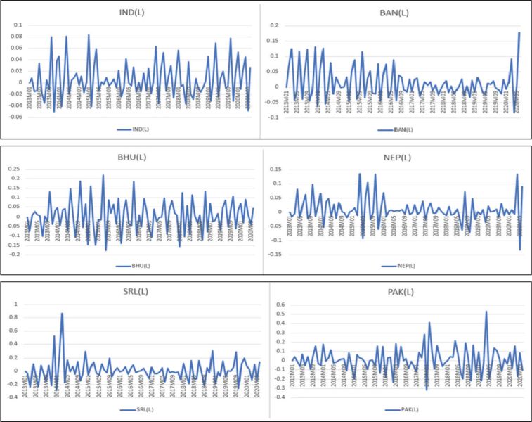
Figures 1–6 presented the export growth rates, and it is evident from seeing them that except for Bhutan, the rest of the nations in the present study witnessed a distinctive downturn in export growth in the early COVID phases.

Figures 1–6. The Monthly Export Growth Rates of LMI South Asian Economies (April 2013 till June 2020).

Source: From extreme left to right on-wards, Figure 1 is India, Figure 2 is Bangladesh, Figure 3 is Bhutan, Figure 4 is Nepal, Figure 5 is Sri Lanka and Figure 6 in Pakistan. Please note that from Figure 1 to 28, the X series denotes the time period in months, and Y denotes the scale on which the values are measured.

It is also visible that there were a lot of upper spikes witnessed within several countries. Nepal’s and India’s export monthly growth, however, remained ‘range-bound.’ While India has seen export growth of less than 10% nearly four times between 2013 and 2019, Bangladesh has seen it 10 times, Nepal 14 times, Sri Lanka 14 times, and Pakistan nine times.

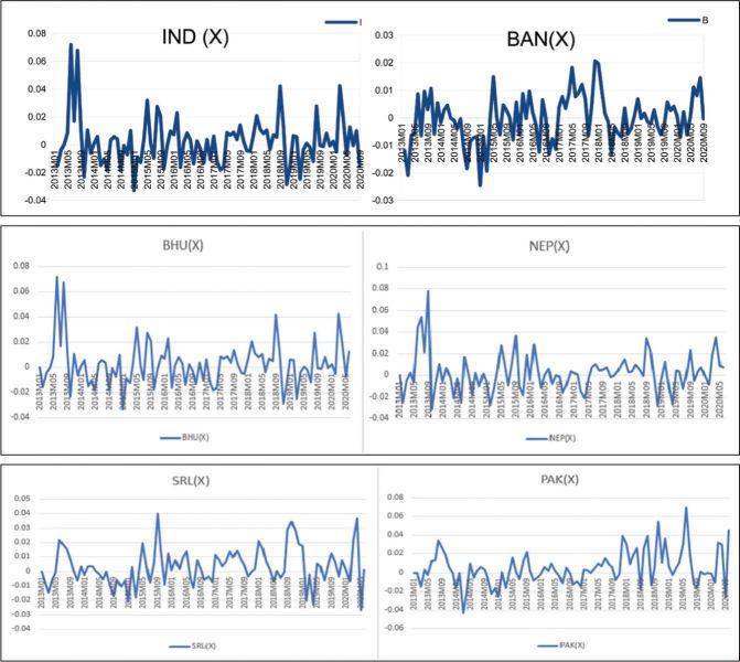
Moving the emphasis towards Figures 7–12 (see page 41), comparing line charts for historical monthly growth rates of imports As can be witnessed, most economies shared a common trait (some sort of consistency or clustering of volatility). Almost all countries experienced a ‘major spike’ in early COVID pandemic episodes. However, some differences can be seen when closely examined. Like India, Bangladesh saw its import growth dip to at least nine times below 10% in comparison to its export growth, and surprisingly, Bhutan, like the export growth figures, shared no sign of a downturn below 10% (within 90 months of study). Nepal experienced it 10–11 times, Sri Lanka experienced a negative drop in imports in the latter half of the period to nearly 9–10 times, and Pakistan experienced it 10 times as its import growth rates fell to negative 10%.

Figures 7–12. The Monthly Import Growth Rates of LMI South Asian Economies (April 2013 till June 2020).

 

As a result, on the time spectrum of monthly growth rates of imports, Bhutan was on one end with no major downturns, while Bangladesh was on the other end with nearly 12–13 downturns in the same time period. India’s position was also very distinctive since, unlike other nations, the drop in import growth rates was 10 times greater than the drop in export growth rates (only 4 times).

Now, in terms of the upswing in the import growth rates, India saw almost ‘none’ of the values move above 20%, Bangladesh’s import growth exceeded 20% nine times, and Bhutan saw significant increases in 2015 and 2017—a total of five times it breached the 20% mark. Nepal also saw a jump in import growth, rising overall 10 times above 20%, followed by Sri Lanka three times, and finally Pakistan only once.

Referring to Figures 13–18 on growth rates and position in terms of international liquidity, almost all countries were found to have significant volatility patterns. However, in terms of ‘range-boundness,’ Sri Lanka and Pakistan appeared to have the highest ranges. Except at the tail end (the early pandemic phase), India experienced downturns of less than 6% throughout the period, as did Bangladesh. Nepal also only dipped below 6% in monthly international liquidity growth once during the pre-pandemic phase, and Sri Lanka around 13–14 times. Maximum downturns occurred 19 times in Pakistan. In the Indian context, India saw its international liquidity growth improve by more than 6% six times; Bangladesh saw a similar jump range until mid-2016; and nearly 11 times during the early pandemic phase. Bhutan witnessed nine instances of international liquidity growth moving up above 6%; Nepal saw it 10 times; Sri Lanka, 20 times; and finally, Pakistan, almost 26 times. Hence, considering the above figures, Pakistan and Sri Lanka appeared to have been most advantageous (or, in other words, poured more than 6% of the previous month’s liquid funds more than 26 times and 20 times, respectively).

Considering this, India played a safer bet on the international liquidity position, while Pakistan saw the other extreme (with upswings 26 times and downswings 20 times).

Figures 13–18. The Monthly International Liquidity Growth Rates of LMI South Asian Economies (April 2013 till June 2020).

 

Figures 18–24 (see below page 43) are the last component in the graphical analysis. In the case of India, SDR exchange rate growth remained within the lowest bounds until mid-2020. Bangladesh experienced a much lower barrier of 2% on both the upside and downside; the country’s growth rate fell below 2% only twice during the 90-month period. Bhutan saw growth trends above 5% till 2013–14. However, it crossed the upper bound; it crossed eight times the 2% mark. and a 2% drop six times in a row. In comparison, Sri Lanka saw eight times above but only two times below, for a 2% range. Pakistan, particularly beginning in 2017, saw higher upper-growth trends in the SDR exchange rate, breaching the 2% bound 13 times and falling four times. Hence, SDR exchange growth rates appeared to be more stable in comparison to the other variable used in the study.

Figures 19–24. The Monthly SDR Exchange Growth Rates of LMI South Asian Economies (April 2013 till June 2020).

 

Objectives of the Study

After some preliminary investigation of facts, it is important to define the objective of this two-regime, two-phase study:

1. Analysing the change in the direction of regime shift covariates corresponding to specific macroeconomic time-varying risk between the early and mid-COVID phases.
2. Examining the impact of post-regime shocks on the specific macro- economic time-varying risk in the early and during COVID phases.

Literature Review

The literature review was studied concerning the institution’s role in managing macroeconomic shocks, followed by more specific positive uncertainty shocks, volatility shocks, COVID-19, conditional trade volatility shocks, and Markov-switching VAR. However, some articles were specifically studied for lower–middle economies in order to meet the requirements of the current study.

Institutions Role

According to Fielding et al. (2012), developing economies face macroeconomic shocks whose impact should be felt by all the member states. In the event of any external policy shocks that have different impacts on different states at the same time, such results may depict ‘welfare losses.’ To ascertain this, a structural vector auto-regression (SVAR) model was implemented. Due to some heterogeneity expected in the SVAR model, further use of the VECM model with a generalised impulse response of exogenous interest rates was explained. The use of a generalised impulse response is invariant to the order of a shock. Bordo (2020) stressed the rule-based monetary approach and extended swap lines to overcome the monetary burden for emerging economies in the early phases of the COVID crisis. Some member states also advocated for an emphasis on a rule-based approach to the free use of the floating rate regime. Bordo (2020) also stressed managing the balance between the exchange rate regime and the early crisis since it does not adjust seamlessly with inflationary pressures borne by the few weak economies. Hence, from a policy perspective, a cooperative move by central banks together with the active release of SDRs by the IMF can be the best way to maintain international liquidity under control, but in both the above articles, such discussions were not made.

Similarly, in terms of central banks’ cooperative role during the early COVID crisis, Bahaj and Reis (2020) established that any Fed cut on extended swap lines will have a direct impact on domestic financial institutions’ international liquidity position. García-Herrero and Ribakova (2020) explained that the floating rate regime can be of support to foreign investors in emerging economies only in ‘normal times.’ MÜhlich et al. (2020) commented on the extent of the use of the Global Financial Safety Net (GSFN) as the distribution is slightly uneven across the world economies.

Diercks et al. (2020) mentioned that any serial uncertainty shocks (positive shocks) across economies in the early crisis phase have serious implications. The empirical argument was that serial uncertainty shocks have similar intensities when they appear consecutively. Bretscher et al. (2019) show how the ‘risk premium channel,’ that is, the impact of higher uncertainty risks, leads to a higher risk premium and a reduction in a firm’s output and production. Ludvigson et al. (2020) explain COVID-19 as a multi-period natural disaster and therefore used multiple shock windows for analysing its impact. Primiceri and Tambalotti (2020) referred to the US economy and considered that post-COVID-19 employment and consumption will remain major concerns. In COVID-19, crisis-based economic forecasts have made careful assumptions, one of which is to ensure that they match the possibility of early recovery in terms of economic numbers through the use of timely policy interventions called ‘diffusion tilting’ in the article. Baqaee et al. (2020) explained the use of non-pharmaceutical interventions, bringing concepts of smart ‘reopening’ of the economy.

Positive Uncertainty Shocks

Mecikovsky and Meier (2014) discussed the positive uncertainty shocks caused by the COVID pandemic, particularly under flexible labour policies and protective (labour frictions) regimes. Baker et al. (2020) used mainly three approaches for uncertainty shocks in terms of the COVID-19 pandemic. For stock market volatility, a VIX index was used. Newspaper-based volatility was employed to historically check the presence of texts containing the COVID-19 pandemic and related news, and finally, surveys were conducted to take first-hand evidence of the business uncertainties surrounding the current pandemic. Their empirical claim was that this pandemic would cause more than half of the contraction in the US economy in the coming years. Bordo and Siklos (2019) deploy Panel VAR on measures like central bank transparency and central bank independence. Early and after the financial crisis across emerging and advanced economies Chong (2011) explained, with the help of stock market data, the use of conditional volatility shocks using leverage and clustering generalisations with GARCH-type volatility estimates. Benigno et al. (2020) examined endogenous macroeconomic models under leverage constraints leading to crisis (where a sudden stop of capital flow acts as binding friction).

However, several papers on the stock market impact of the COVID-19 crisis concerning conditional volatility and related shocks have emerged since 2019, so it is important to discuss some of them. Borkowska and Hau (2020) described the various forms of conditional volatility models and the standard battery of tests for checking the normality of residuals and stationarity in the various stock prices of designated companies. Liu et al. (2020) explained the volatility spillover and shock effects of the switching GARCH model in their work. Castillo et al. (2020) applied the EGARCH volatility model to various international stock exchanges and stock prices and back-tested the value-at-risk.

Markov Switching VAR

The exogenetic assumption associated with Markov switching was relaxed by Kim et al. (2008). They considered that in the case of ‘early regime shifts,’ there is a parameter instability due to which any serially dependent (like I took the conditional volatility function) or auto-correlated function can assist in an endogenous switching approach. Mishra et al. (n.d.) compared the GST and demonetisation eras with the recent COVID-19 using the Markov-switching VAR method. Bluwstein (2017) showed, through the use of the Bayesian MS-VAR methodology, that financial shocks have asymmetric effects. Çifter (2017) used three regimes, that is, recessionary, moderate, and expansionary phases while dealing with the Fisher equation (inflation affecting the nominal interest rates) and stock markets. According to the paper by Hamilton (1989) and as further corroborated by Çifter (2017), a typical Markov process is a first-order auto-regressive process. Essentially, the probability of a transition or switch happening at any ‘differentiable time component’ in between two time periods is not known in advance. And, second, where there have been strong or weak transition effects across the multiple regimes is also difficult to ascertain.

Overall, after a detailed review of past work in terms of institutions’ roles during crises, the extent of positive shocks and their impact, and the application of Markov-switching vector autoregressive models, It was observed that the studies on the COVID time period with reference to determining time-varying regime shifts with the MS-VAR modelling framework were very rare. Furthermore, no such paper accounted for the ‘change in direction of covariates’ across regime shifts as a determinant of greater trade-related risks in the country. This provides a very novel idea for me to take this work further and come out with some interesting and useful empirical outcomes.

Methodology

The entire data was captured in a spreadsheet from the World Trade Organisation (WTO) website database. The research used four endogenous variables, namely exports, imports, international liquidity, and SDR exchange rates, and all figures were in million US dollars converted to growth rate percentages, excluding the scale and unit effect. The period chosen was from January 2013 to June 2020 on a monthly basis. The selection of this time frame was motivated primarily by two factors: first, it covered a significant period prior to the implementation of COVID in December 2019. And, from 2013 on, events like Brexit, the Indo-China trade war, and some other global and regional shocks also impacted the South Asian economies.

For conditional volatility (on an annual basis), the use of an exponentially weighted moving average (in short, EWMA) was employed, where the decay rate was kept at 0.97. In this article, a two-phase study has been conducted,

The first phase (or pre-COVID phase) is when we included April 2013 through November 2019 in the first differences of logarithmic EWMA volatility figures, and the other one is where the early-COVID period was also added, that is, April 2013 through June 2020 (a total of 7 months of the pandemic were included). Hence, this study used two phases with unequal periods.

The method adopted can be explained in the following steps:

• First, the exponential weighted moving average (time-varying volatility) was calculated for all four macroeconomic indicators and with respect to six economies.
• Second, after gathering the exponential weighted moving average time series, the unit root test was conducted.
• Third, the Markov-switching (mean) Vector-Autoregressive model was implemented.
• Fourth, the corresponding shock response data was gathered.
• Finally, the direction and reversion time of the two-phase regime-shift covariates were examined.

Graphically, it can be presented like this:

 

Results

Test of Unit Root

Table 1 depicts the unit root results, which were applied uniformly to the first differences of logarithmic conditional volatility. As can be seen, for all six countries (currently for export data), there are no unit root properties exhibited.

Changes in the direction of regime-shift covariates during the early and late COVID phases, as well as the corresponding shock responses (in relation to India’s time-varying volatility predictions).

Only if the covariates or coefficients associated with early-COVID and during-COVID phase regime shifts (i.e., Regimes 1 and 2) change direction under both phases can empirically be analysed. Then only such countries have a significant impact on the time-varying volatility of the underlying macroeconomic indicator. What it also means is that since the direction of regime coefficients or covariates is altered in both phases, which means that the COVID impact on certain nations has not been discounted in exports, imports, international liquidity, and SDR-associated exchange rates’ time-varying volatility. As a result, predicting a higher variance in the dependent macroeconomic volatility over time is more difficult. The same can be said of the shock responses in terms of their reversion period. In this case, as in the preceding preposition, if the regime shifts for the early and late COVID phases, the recovery time period for both phases changes. It clearly indicates a more volatile state of underlining macroeconomic dependence and time-varying volatility.

Hence, all the respective tables are divided into two sets of analysis:

First, for understanding the countries whose covariates changed with regimes across two phases, And then a similar analysis was conducted for shock impulses and their reversions.

Accordingly, looking at the results from Table 6, Table 8, Table 10, and Table 12 simultaneously, India’s chances of experiencing higher time-varying export and import volatility are Nepal’s time-varying export volatility regime shifts and their direction should be taken into empirical consideration. Similarly, Bangladesh’s and Bhutan’s time-varying international liquidity volatility is a concern for India’s time-varying international liquidity volatility.

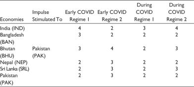
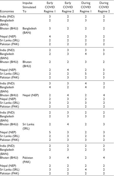
Further, in terms of shock responses, particularly the reversion time period, It can be seen through Table 7, Table 9, Table 11, and Table 13 that when the 1-SD shock was provided to India’s time-varying export volatility, we could visualise the ‘inconsistencies in the recovery period’ (with reference to change in the post-shock recovery time period across two phases between the regime shifts) for Bangladesh, Bhutan, and Nepal. While, in the case of India’s shock response in terms of time-varying import volatility, inconsistencies were observed with countries like Bhutan and Nepal. Further, in terms of a 1-SD shock to India’s time-varying international liquidity volatility, Sri Lanka’s recovery responses were inconsistent. And finally, with respect to India’s time-varying SDR exchange rate volatility shock, none were seen to have inconsistencies across both phases.

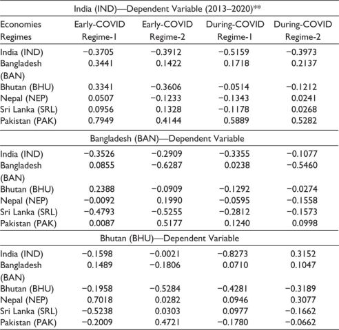
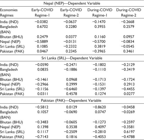
Table 6. Markov-switching (endogenous switching means) VAR Coefficients for Export Volatility Series*.

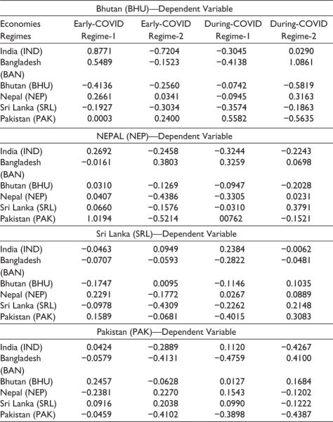
Notes: *Here, the VAR coefficients are for the first lag values of the first differences of logarithmic volatility.

**Period is 2014-01 to 2020-06 (78 monthly values for the early COVID phase and 71 monthly values for the pre-COVID phase).

Table 7. MS-VAR Impulse Response for Export Volatility Series*.

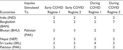
Note: *Initial shock recovery period (in months).

Table 8. Markov-switching (endogenous switching means) VAR Coefficients for Import Volatility Series*.

Notes: *Here, the VAR coefficients are for the first lag values of the first differences of logarithmic volatility.

**Period is 2014–01 to 2020–06 (78 monthly values for the early COVID phase and 71 monthly values for the pre-COVID phase).

 Table  9. MS-VAR Impulse Response for Import Volatility Series*.

Note: *Initial shock recovery period (in months).

Table 10. Markov-switching (endogenous switching means) VAR Coefficients for International Liquidity Volatility Series*.

Notes: *Here, the VAR coefficients are for the first lag values of the first differences of logarithmic volatility.

**Period is 2014-01 to 2020-06 (78 monthly values for the early COVID phase and 71 monthly values for the pre-COVID phase).

Table 11. MS-VAR Impulse Response for International Liquidity Volatility Series*.

Note: *Initial shock recovery period (in months).

Table 12. Markov-switching (endogenous switching means) VAR Coefficients for SDR Exchange Rates Volatility Series*.

Notes: *Here, the VAR coefficients are for the first lag values of the first differences of logarithmic volatility.

**Period is 2014-01 to 2020-06 (78 monthly values for the early COVID phase and 71 monthly values for the pre-COVID phase).

Table 13. MS-VAR Impulse Response for SDR Exchange Rates Volatility Series*.

Note: *Initial shock recovery period (in months).

Since similar ‘p’ values appeared for the rest of the four macroeconomic variables, their results are not depicted.

Discussion

Corresponding to the above analysis and specifically with reference to the Indian economy It has been observed that trade-related (import and export) time-varying volatility will be deeply affected by the change in the direction of regime shifts between the two phases of Nepal’s time-varying export and import volatility. With reference to shock responses by time-varying India’s export and import volatility, Bhutan and Nepal’s time-varying export and import volatility had dissimilar reversion periods in both phases (i.e., early COID and during COID). Hence, this empirical work opens an interesting dimension towards studying the patterns of ‘change in direction of the covariate of regime shifts’ as the key learning that can propel the intensity of variability or volatility in the dependent variable series. On the contrary, any stable movement of a covariate across phases usually makes the forecast predictable, and thus any of India’s trade policies face fewer challenges of knee-jerk reactions. During the COVID period, the countries’ trade volatility responses were found to have had some intense impacts on India’s trade volatility in the past. And as explained, any change in the direction of the regime shift coefficients will further exacerbate the situation.

Conclusive Remarks

Countries with strong trade relations must use tools like Markov switching in advance to ensure that any regime shift patterns can help the countries plan their future course of action in terms of trade-related risks. It is also important that international liquidity and SDR exchange rates be independently studied in order to see their role in managing trade-related imbalances.

Limitations

One of the major limitations was that this study only took the two phases, that is, early COVID and COVID, as an arbitrary measure. Hence, a more scientific basis for such classification may be needed. The study focused on India’s changing relationships with its member countries in terms of trade, liquidity, and exchange rate-related measures over time. Finally, the duration could have been extended. In addition, after leaving COVID, other local (country-specific) factors could have been studied while the regime shifts covariates were observed.

Remedies to Overcome Limitations

Significant advances have been made in the preposition of using ‘change in the direction of covariates of regime shifts across two phases’ as the sole outcome defining the extent of increased probability of trade-related volatility in India. It is therefore essential that a more robust and extensive sample period and countries be utilised for the study to make the statistical proposition more generalised and theoretically validated.

Furthermore, previous research on trade-related risks employed time-varying techniques like autoregressive distributed lag regression. Such techniques must have been compared to ensure the superiority of Markov-switching vector autoregression for this study.

Scope

This work can be used by policy experts who are dealing with trade-related risks and other international trading firms in terms of managing their cash flows and hedging using the above model outcomes. Moreover, macroeconomic analysts and modellers may find the use of ‘change in direction of regime shift covariates across two phases’ a very useful and novel idea to predict early signals in terms of trade-related shocks in the economy. Besides, this study can be easily extended for multiple countries’ trade data and other stylized shock responses.

Policy Implications

From the standpoints of trade policy and macroeconomic policy, this study explains why, during times of economic stress, closely-knit trading countries should avoid trade-related risks when they anticipate an alarming sign of time-varying regime shifts. Such studies, therefore, have very useful applications for early warning signals, particularly in reference to trade-related shocks, which can appear in the early, middle, or late stages of economic stress.

Declaration of Conflicting Interests

The author declared no potential conflicts of interest with respect to the research, authorship, and/or publication of this article.

Funding

The author received no financial support for the research, authorship, and/or publication of this article.

ORCID iD

Rohit Malhotra https://orcid.org/0000-0002-4801-0916