Introduction

India has an extensive coastline of approximately 7,517 km along nine coastal states: Gujarat, Maharashtra, Karnataka, Goa, Kerala (west coast), Tamil Nadu, Andhra Pradesh, Orissa and West Bengal (East Coast). There are 12 major ports and docks and over 200 minor ports. Of the 12 major ports, six are on the west coast (Kandla, Mumbai, JNPT, Mormogao, Cochin and New Mangalore) and six on the east coast (Chennai, Ennore, Tuticorin, Paradip, Visakhapatnam, Kolkata, Chennai, Mumbai and Mormogao ports are over 100 years old. Kolkata port has two major dock systems, one at Kolkata and the other at Haldia. JNPT started its operation after 1989. Ennore port (now known as Kamarajar port) is the 12th major port that started operation in 1999. Ennore port is the only port in India registered as a company, and others are governed by the Major Ports Act. Approximately 95% of India’s trading volume and 70% by value are done through maritime ports.

After liberalisation in 1991 and the emergence of the global production process, commodity exports very quickly increased manyfold through the seaports and forced countries worldwide to undergo port reforms. India is no exception. Previous showed that not all privatised ports were equally efficient, and some performed poorly compared to government-run ports (Dasgupta & Sinha, 2016). Another work (Sinha & Chowdhury, 2018) showed that given the pension and fixed cost burden of Indian ports, not all terminals or services should be privatised.

In the last decades, general awareness about the impact of port performance and efficiency on trade has increased partly due to numerous reports on the fragile state of Indian port infrastructure. India started the reformation process to enhance the performance and productivity of its ports through some development programs (PIB, 2015; PIB, 2011; Ministry of Ports, Shipping and Waterways, 2016). It includes taking measures like––adopting the landlord port model and outsourcing some of its cargo handling operations to private players, capacity expansion and dredging activities to increase the draft depth to accommodate larger ships, introducing containerisation, replacing obsolete and poorly maintained equipment, installing modernised equipment, reducing excessive labour and the intervening of trade unions and labour strikes.

The four major performance indicators for Indian ports are ship turnaround time (TRT), idle time in percentage (IT%), pre-berthing delay (PBD) and output per ship-berth-day (OSBD).

The basic definitions for these performance indicators as stated in the Basic Port Statistics Report (2020–2021) of the Ministry of Shipping, Government of India, as below:

1. Turnaround time: Total time a ship spends (in days) from pilot boarding to de-boarding.
2. Output per ship-berth-day: Total tonnage handled distributed over the total number of berth days
3. Idle time percentage: Percentage of non-working time of a ship (without loading or unloading of cargo) at berth.
4. Pre-berthing delay: The time (in days) a ship waits before entering a berth.

The functional values of the above indicators give a fair and reasonable picture of port performance. It is necessary to reduce TRT, PBD and IT and to increase OSBD for a port to operate efficiently and increase its productivity and market share of port throughput.

Previous studies show (Chakrabartty & Sinha, 2022; Nayak et al., 2022) that a composite indicator leads the way for port planners to delve down into the cause of inefficiency or other performance, for example, sustainability (Sinha & Chowdhury, 2020). However, there is an insignificant reference to studies that compared the performance of ports over different periods and amongst those that shared a common hinterland––competing with a common customer base or cargo source. Periods refer to the time when different reforms were initiated and whether such measures did impact port performances.

Over the last 20 years, the Indian government has implemented several reforms. Since 2005, various port infrastructure and institutional development initiatives have been taken. These include ‘The National Maritime Development Programme’ (PIB, 2015), the ‘Maritime Agenda 2010–2020’ (PIB, 2011) and reforms in ‘Major Port Authorities Act-2021’ (NIC, 2021).

In 2016, Customs and Indian Ports introduced measures to minimise the dwell time of containers. These schemes included Direct Port Delivery (DPD) and Direct Port Entry (DPE) for import and export containers. Under the DPD scheme, an importer can clear the container at a port without routing it through container freight stations (CFS). DPE allows export containers stuffed at a factory or exporter’s warehouse to be self-sealed and move to port directly without touching inland container depots (ICDs) or container freight stations (CFS; Shipping Ministry, 2021).

Under Maritime India Vision 2030, the Government of India initiated investments (worth 6 Trillion USD) in enhancing port capacity under the initiative called Sagarmala. The aim is to achieve a capacity of 3,300 Million Tons per annum (MIV, 2021).

However, the share of major ports continues to slide—it had a 90% share in 1950 and reduced to less than 50% in 2019. The traffic handled by non-major ports (613 million tons) exceeded the handling by the major ports (575 million tons) in 2019 (refer to https://timesofindia.indiatimes.com/blogs/voices/what-future-holds-for-maritime-logistics-in-india/). The ports in India could not match the performance levels of many other ports in Asia and around the world. In 2022, the average turnaround time (ATRT) in Indian ports was around 2.18 days (Basic Port Statistics Report, 2021), as against 0.34 days in a Japanese port, 0.62 days in Chinese ports, 0.8 days in Singapore port and Netherlands ports and 0.7 days in UK ports (Statista.com).

Existing researches (Nayak et al., 2022) on major Indian ports show their performance comparisons and consider financial performance as the output affected by the physical, socioeconomic and operational efficiencies. This study has three major limitations—one: financial performance can improve with an increase or articulation of port tariff; two: port performance affects the primary stakeholders— ships and shippers—not considered for research validation and three: the existing study does not consider that government reforms aimed at improvement of port performance.

Thus, there is a need to consider the impact of port performance on ship calls. The stakeholders’ decision to prefer one port over the other is reflected in the number of ships visiting the port. If performance deteriorates, the ships and shippers will avoid such ports. Second, whether government reforms impact the port equally or partially may vary with the degree of its implementation by individual port authorities.

This article aims to answer two research questions:

RQ1: Have port reforms improved port performance?

RQ2: Do ports with overlapping hinterlands compete, or does one port’s performance complement the other?

The authors developed a composite port performance index in this article and compared port performance across different periods. It also showed how operational performance affects the number of ships calling at the port.

This article has seven sections. The next section describes the objectives in detail, and the third section discusses the extant literature. The fourth section describes the methodology and the results are discussed in the fifth section. The sixth section analyses the managerial implications of the findings, and the seventh section concludes the research work and states the limitations.

Objectives

There are two main objectives of this article:

1. The first objective is to compute a composite port performance index (PPI) using principal component analysis (PCA) for all the major ports. A composite port performance indicator is necessary, as different ports perform differently in terms of performance indicators, and it becomes difficult to benchmark the ports based on individual performance indicators.

       The PPI comprises the four important performance indicators––TRT, PBD, OSBD and IT%. The average value (annual) of these indicators has been considered for the study.

2. The second objective is to use the composite performance index to assess the effect of the port performance on the number of vessels (port calls) for the ports using breakpoint regression analysis (segmented regression analysis).

For the second objective, we have restricted to three ports––Paradip, Visakhapatnam and HDC (Haldia port). The article uses breakpoint regression analysis (segmented regression) to capture the effect, considering ‘time’. These three ports are all on the eastern coast of India. These three ports primarily handle bulk cargo, such as coal and iron ore, and share an overlapping hinterland. Thus, the hypothesis is: Ports sharing a common hinterland always compete with each other—RQ2.

Literature Review

Research articles on assessing the relative performance of Indian ports based on performance indicators and composite performance index over different periods are scarce. Very few articles also find a causal relationship between port productivity or port calls (number of vessels) and performance indicators in the Indian context.

De and Ghosh (2003) tried to uncover the long-term and short-term causal relationship between port performance and port traffic individually for all the major ports in India using co-integration analysis and Engle Granger causality, two important tools used in econometrics from 1985 to 1999. They have derived the composite performance index for each port using operational indicators like average turnaround time (ATRT), PBD, idle time percentage, OSBD, berth occupancy rate, berth throughput rate and financial indicators like operating surplus per tonne of cargo handled. In the case of most of the ports, they found either weak or strong causality or no causality with direction from performance to traffic.

Dayanand and Dwarakish (2018) examined the correlation between port productivity (port throughput volume) and performance indicators like ATRT, average pre-berthing delay, average output per ship-berth-day, idle time percentage, average output per hook per shift and number of vessels (port calls) for New Mangalore port for the period 1990 to 2014. Idle time percentage, turnaround time and pre-berthing delay have a negative correlation with productivity, and the rest have a positive correlation.

(Mandal et al., 2016) ranked the Indian ports by constructing a composite PPI and grouping the ports based on hierarchical clustering. The basic performance indicators were turnaround time, pre-berthing delay, average output per ship-berth-day and idle time percentage. Instead of using TRT and PBD directly, they have created a ratio of TRT and average output per ship berth day to compute the ATRT and a ratio of PBD and average output per ship-berth-day to compute a new variable detention time to output ratio (DTOR). The weights for the performance indicators have been derived using Analytic Hierarchy Process.

Solanki and Inumula (2020) have ranked the major Indian ports by constructing a composite PPI, using key performance indicators like TRT, PBD, OSBD and IT percentage as components using PCA to give weights to the indicators. Data for the period 1999 to 2017 was used for the analysis. JNPT port occupies the first position, followed by Ennore port in the second rank and Kandla port in the third position. Kolkata, Haldia and Tuticorin demonstrated poor performance and ranked in 13, 12 and 11th positions, respectively. Kumar (2022) extended the same method by Dayanand and Dwarakish (2018) to all the major ports of India using Pearson correlation analysis using data between 2007 and 2019.

In recent work, Nayak et al. (2022) computed a unified PPI based on the quantile approach and compared it with the PCA method. The article established the relevance of the indicator by showing its positive relationship with the financial outcome of the ports. This article validated its method on the Indian ports. The results may stand negated if ports increase their tariff and service charges. Besides, ports do not share the same hinterland, so its comparison with all ports for all cargo may not reflect the right rankings. In this article, a comparison of ports sharing a common hinterland has been made.

Choosing the right output variable is crucial for measuring port performance (Dasgupta & Sinha, 2016; Sinha & Dasgupta, 2017). The impact of performance affects ship calls, which impacts cargo throughput. This article tests the effect of port performance on ship calls based on the port performance scores and ship calls over time.

Research Methodology

This section is divided into three subsections. In the first subsection, a box plot analysis, for all the major ports, has been carried out to show the initial findings about port performance regarding four crucial operational performance indicators. The second subsection discusses the development of a composite indicator—the PPI. The third subsection illustrates the use of breakpoint regression analysis to validate the relationship of port performance with ship calls.

Annual data for the period 1999 to 2000 to the year 2020 to 2021 has been selected for the study. The sources of the data are:

1. Basic Port Statistics reports (MoS) for data from FY 2008 to 2020
2. Data from 1999 to 2007 were compiled from the works of Solanki and Inumula (2020).

Initial Box Plot Analysis of the Performance of the Major Ports

Figure 1a and Table A1 show that JNPT has the least ATRT (1.23–2.54 days) with the least variance in ATRT value. The next best level performers, after JNPT, are Cochin (1.45–3.54 days), New Mangalore (1.90–3.80 days) and Kamarajar port (1.72–4.24 days). Mormugao port (2.33–8.91 days) is the worst performer, followed by Kandla port (2.45–7.26 days). HDC (2.75–5.47 days) outperforms KDC (3.17–6.80 days). Visakhapatnam (2.43–5.84 days), Paradip port (2.34–7.01 days), Chennai (1.98–6.40 days), Tuticorin (1.67–4.94 days) and Mumbai (1.70–5.60 days) are performing approximately at the same level. The outlier values of the indicators, shown in Figure 1, have been excluded.

Figure 1. Box Plots of ATRT, APBD, AOSBD and IT%.

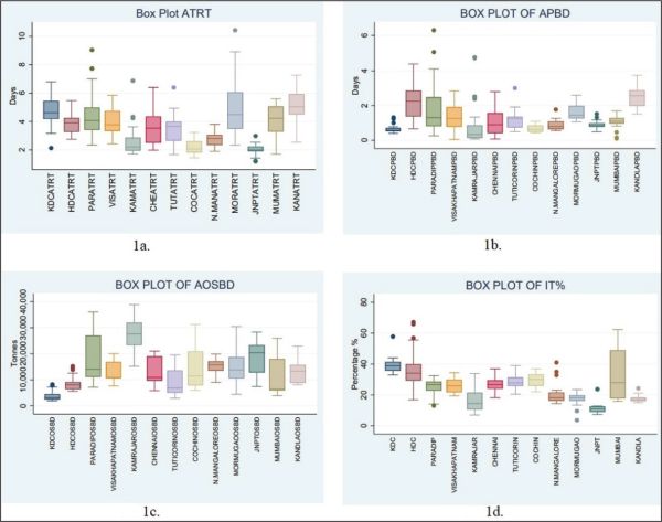
Source: STATA 16 (trial version).

 

Figure 1b and Table A2 show that Kamarajar port (0.07–2.38 days), Kolkata (0.4–1.1 days) and Cochin (0.43–1.09 days) are at the top levels of performance, followed by JNPT (0.49–1.17 days). New Mangalore (0.55–1.26 days) and Mumbai port (0.10–1.41 days) are at the next best level of performance. Paradip port (0.26–4.11 days), Visakhapatnam (0.07–2.84 days) and Mormugao port (1.06–2.59 days) have APBD at approximately the same level. HDC (0.66–3.73 days) and Kandla Port (1.51–3.74 days) have high APBD.

Figure 1c and Table A3 demonstrate Kamarajar port has the best performance in terms of OSBD (15,149–38,871 tonnes). JNPT (7,391–28,296 tonnes), Paradip (7,106–36,030 tonnes) and Cochin (5,979–31,258 tonnes) also performed well. The worst performer is Kolkata (1,918–7,765 tonnes), HDC (5,599–14,223 tonnes) and Tuticorin (2,891–19,494 tonnes) are just above Kolkata in OSBD performance.

Figure 1d and Table A4 show that in terms of idle time percentage, KDC (32.9%–44.0%), HDC (16.9%–55.6%) and Mumbai (15.9%–62.4%) are much higher than other ports. JNPT (7.4%–23.7%) is the best performer (7.4%–12.9%). Other ports are more or less at the same level of performance.

Figure 2. PCA.

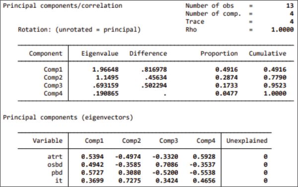
Source: STATA 16.

 

From the above analysis, it is apparent that ports perform differently with reference to different performance indicators. Box plots only preliminarily indicate the performance of a port for an individual indicator in a time-invariant manner. It cannot capture the overall performance of a port relative to other ports, with all performance indicators with reference to time, and hence, there is a need to determine a single composite PPI that reflects performance variation, in all four indicators.

In the next section, we will construct a Composite Port Performance Index (0–100 scale, 0 refers worst performance and 100 is the best performance) from the above four performance indicators.

Principal Component Analysis

A composite index is constructed by combining several variables or indicators. Composite indices can summarise multi-dimensional issues (Saisana et al., 2005). The literature on composite indicators is vast. Composite index has been widely used in many fields, including social sciences (Booysen, 2002), healthcare, environmental science, economy, technological development and human resources. For example, the Health System Achievement Index adopted by WHO (Reinhardt & Cheng, 2000), the Internal Market Index in the field of Economy (Tarantola et al., 2004), the Information and Communication Technology Development Index in the field of Information and Communication Technology adopted by International Telecommunication Union in 2009 and revised in 2020, Human Development Index adopted by United Nations Development Programme is a widely known index to assess human development, combining indicators of health, education and income.

In the port sector also, several composite indicators are used, for example––

At the country level, liner shipping connectivity index (Niérat & Guerrero, 2019) indicates how well countries are connected to global shipping networks. It computes the index based on six components of the maritime transport sector, namely the number of ships, ships’ container-carrying capacity, maximum vessel size, the number of services, the number of country pairs with a direct connection and the number of companies that deploy container ships in a country’s ports.

PPI of container handling ports (World Bank, 2022) is computed primarily combining FA (factor analysis) and administrative approach (expert judgment). The index is based on the comprehensive measure of port hours per ship call determined bygreater or lesser workloads and smaller or larger capacity ships; calls are analysed in 10 narrow call size groups and five ship size groups that generally reflect the types of ships deployed on specific trades and services.

The most important part of a composite PPI is allocating weight to individual port performance indicators. Popular methods of weight are mathematical formulas, AHP and principle components. Weight by the AHP method is subjective and ad-hoc, resulting in biased and unwarranted results.

In this article, the composite PPI is constructed in the following steps:

Step 1: Raw data is normalised according to the following formula

1.     If the higher value of a variable is better, then the formula for transformation is

                                                             

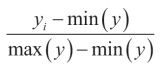
        The higher value of OSBD is better.

2.     If the lower value of the variable is better, then the formula for transformation is

                                                                                                                          

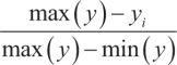
        The lower value of ATRT, APBD and IT(%) is better.

Step 2: Year-wise values of the four variables ATRT, AOSBD, APBD and IT(%) are collected and PCA is applied to the normalised data.

Step 3: The weights for a particular year are derived using the formula––

                                                (1)

Where (i) denotes a particular indicator variable, loadingij is the loading value of i^th indicator on its j^th principle component. Eigenvalue_j is the eigenvalue of the j^th principle component. Principle components with eigenvalues greater than or equal to 1 are considered.

Step 4: Final PPI for a port, from 1999–2000 to 2020–2021 is calculated using formula -

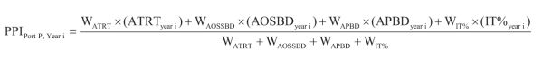
                                                                                                                                                                                     (2)

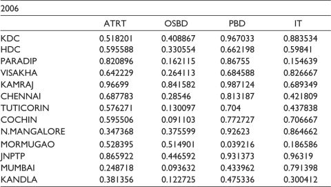
We illustrate Step 1 to 4, with year 2006 data (Table 1).

Table 1. Raw Data for All the Indicators for Year 2006 Weight Calculation for Illustration.

 

The scree plot (Figure 3) shows two components having eigenvalue greater than 1. Hence, two components have been used to calculate the weight of 2006.

Figure 3. Scree Plot for Illustration.

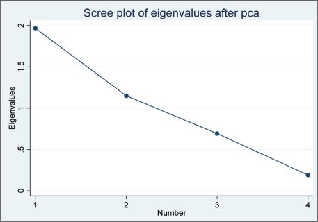
Source: STATA.

 

Equations (1a.) to (1d.) calculate the weight for the performance indicators for the year 2006 using Equation 1.

                                                       (1a.)

                                                               (1b.)

                                                                (1c.)

                                                               (1d.)

The weights, computed for the rest of the years, are shown in Table 2. Using Formula (2), PPIs for each port for all the years are calculated and tabulated in Table 3. Year-wise ranks of the ports are shown in Table 4.

Table 2. The Time Varying Weights of All Performance Indicators (1999–2000 to 2020–2021).

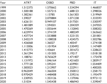
Source: The authors own computation in STATA.

Table 3. The Port Performance Index for the 13 Major Ports.

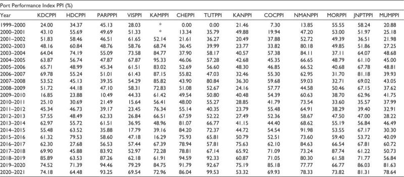
Note: *represents the port not under operation.

 

Table 4. Rank Based on the Port Performance Index for the 13 Major Ports.

Note: *represents the port is not under operation.

To assess the relative performance of each of the 13 major docks with respect to its own performance over the years, a standardised port performance index (SPPI) (Mandal et al., 2016) for each port is constructed based on formula (3) and the result is tabulated in Table 5.

Table 5. Standardised Port Performance Index (SPPI) for the 13 Major Ports.

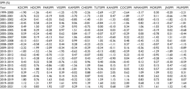
Note: *represents the port not under operation.

 

                                                       (3)

SPPI = 0 means average performance, and SPPI > 0 is below above average performance, while SPPI < 0 means below average performance.

The data from 1999 to 2020 was considered for 13 ports and dock systems with four variables. Thus, the dataset constitutes secondary data; hence, the sample size is fixed and cannot be varied by including higher responses as in the primary survey. In any case, in this study, the KMO values ranged around 0.6, indicating the acceptability of findings with some exceptions. The findings were validated with box plot and regression analysis.

Breakpoint Regression

A linear regression model explains the dependent variable y in terms of the independent variable x in the form:

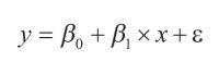                                                                    (4)

b₀ is the intercept and b₁ are coefficient of x₁, respectively.

f represents the unobserved random variable component. The linear regression model above assumes that the parameters b₁ of the model do not vary across observations.

In the case of time series data, the series may reflect abrupt change at a single point or multiple points in time in trend or intercept or both. These time points are known as ‘structural breakpoints’. If there are T breakpoints, there must be T + 1 segments.

With structural breaks, the assumption of non-variance of the parameters of a simple linear regression model holds no more. Coefficients vary from segment to segment. This type of regression model is known as a ‘segmented regression model’ or sometimes termed as ‘breakpoint regression model’ in econometrics.

For illustration, consider there is a single breakpoint T in the dependent variable. Therefore, the linear regression equation (1) now breaks into two equations as:

                                                (5)

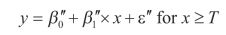                                               (6)

The procedure for breakpoint regression can be divided into two steps:

1. Single or multiple breakpoint detection in dependent series.
2. Fitting equations in the form of (5) and (6) with the usual procedure of linear regression.

The studies on structural break began with the work of Gregory Chow (1960). The Chow test is applied in the data series if a single break date is known. In the late 1970s and early 1990s, many researchers have worked on estimating unknown single breakpoint in time series (Andrews, 1993; Bai et al., 1998; Banerjee et al., 1992; Brown et al., 1975; Hansen, 1992; Perron, 1989, 1990; Zivot & Andrews, 1992). The focus was not only on estimating the break dates but also towards evaluating the stability of the estimated coefficients, detection of serial correlation, unit root and heteroskedasticity in residual terms of the model, which affects the stability of the regression model in whole. In economic time series, multiple breakpoints are quite common. (Bai, 1997; Bai & Perron, 1998) have significantly contributed to the literature by suggesting some procedures, popularly known as Bai-Perron class of tests, to estimate multiple breakpoints in time series using global maximiser, sequential analysis and hybrid method employing both global maximiser and sequential method.

The breakpoint regression analysis can be performed with coefficients that are ordinary least squares. However, the reliability of the coefficients may be in question if the time series have serial correlation and heteroskedasticity in the errors. In this case, the estimation method proposed by (Newey & West, 1987) may be used, which estimates robust coefficients using some non-parametric adjustments (pre-whitening the residuals) to the coefficient covariance matrix.

The coefficients estimation can be done assuming homogenous error variances with a common distribution across regimes or error variances that are different across regimes.

We have carried out the segmented regression (breakpoint regression) in the following steps:

Step 1: Maximum of three breakpoints are determined using ‘Bai-Perron test of 1 to M globally determined breaks’ with unweighted Max F method. N breaks generate N + 1 segments.

Step 2: For each of the N + 1 segments, a linear fit equation of the form y = mx + c is generated. The coefficients of the model and the intercept terms are generated not using the ordinary least square method but using HAC or Newey and West method, which considers heteroskedasticity and serial correlation in the model.

Step 3: The derived model is tested with Jarque–Bera test of normality, Breush–Pagan test of the presence of serial correlation (specifying lags in the model), Durbin Watson test of Serial correlation (without lag in the model) and Breusch–Pagan–Godfrey test of heteroskedasticity.

A model is selected only if the R-square is sufficiently high, residuals are free from serial correlation and heteroscedasticity and the residual distribution is normal. Durbin Watson value is between 1.50 and 2.50.

In this article, we have used breakpoint regression analysis on a dataset for 20 years (1999–2020) to find out whether the PPIs of HDC, Visakhapatnam and Paradip ports affect their number of vessels, significantly. The models are specified the sixth section.

Results and Discussion

PPI, SPPI and Box Plot Analysis

PPI for all the major ports computed using Equation (2) is listed in Table 4.

Figure 4 is divided into two sections—Figure 4a (1999–2000 to 2009–2010) and Figure 4b (2010–2011 to 2020–2021)—to understand relative performance change in terms of rank (change in box plot levels) for the ports. Kamarajar port (KAM), the best performing port in 1999–2010, is no longer the best-performing port in 2010–2020 as its rank varies with a large IQR, meaning that its performance is no more consistent. Chennai port (CHE), poor-performing port from 1999 to 2010, has improved its performance to a significant level and the rank variation has also reduced to a great extent showing consistently well performance. Rank of JNPT has also gone down from 2010–2020. New Mangalore port (NMAN) has also improved its performance. Rank of Kolkata port (KDC) and Mumbai port (MUM) has not changed much in the two-time ranges. Performance of Visakhapatnam port (VIS) and Haldia port (HDC) have deteriorated.

Figure 4. Box Plots of the Ranks of Ports Based on PPI.

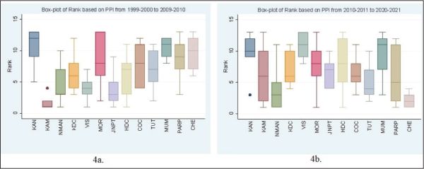
Source: STATA 16.0.

 

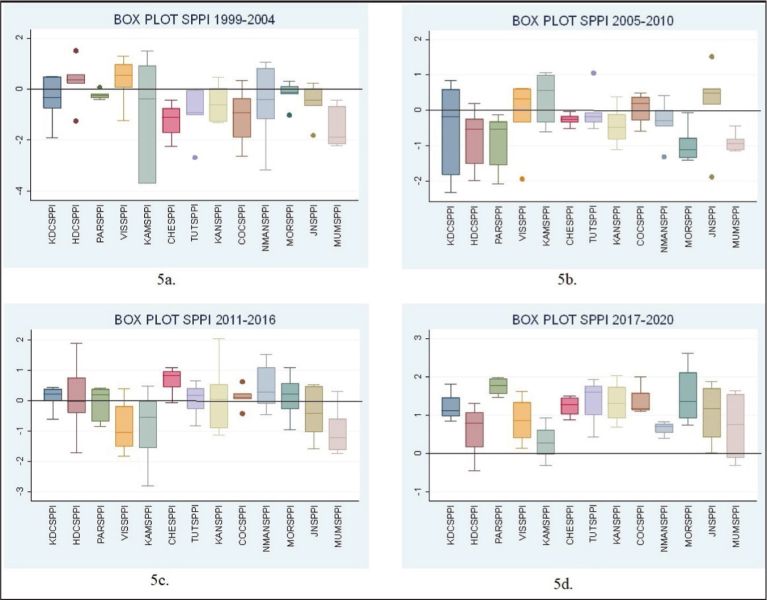
Figure 5 shows the performance change of each port relative to its performance. From Figure 5a to 5b, it is evident that most major Indian ports performed below average. Some improvements are visible to some extent in Figure 5c and finally in Figure 5d. In time period 2017–2020, all the ports performance has improved significantly above average with Paradip port being the best performer, followed by Cochin port and Chennai port in the second position. The worst performers are HDC, Mumbai and Kamarajar ports.

Figure 5. Box Plot for SPPI Divided Into Four Time Periods—(1999–2004), (2005–2010), (2011–2016) and (2017–2020).

 

In 2005–2006, the Central government formulated the National Maritime Development Programme to augment the capacity of the major Indian ports and improve their performance by 2012. For this, an investment of 55,800 crore was planned. Focus of the programme was also to improve the service quality of the ports by carrying out operations at ports under PPP mode.

To assess the progress, a performance analysis of the functioning of major Indian ports was conducted by the Comptroller and Audit General of India on behalf of the Ministry of Shipping, GOI in 2009, report number 3 (CAG, 2009).

The major findings of the audit were:

1. Lack of navigable draft depth—Most of the major ports of India, except Chennai, New Mangalore and Visakhapatnam, lacked navigable draft depth at their channels which barred larger vessels with dead weight tonnage greater than 60,000. The situation was worst for KDC and HDC, where more than 21% of the vessels were to be lightened to access the berths.
2. High pre-berthing delay, except Visakhapatnam port, the significant pre-berthing delay was observed in all ports due to a lack of specialised berths and a delay in providing pilotage to incoming vessels, leading to high congestion of vessels. It was estimated that maritime trade loss amounted to 1,400 crore per year due to pre-berthing delay.
3. High turnaround time—In most ports, less than 8% of the berths had specialised equipment and mechanised berths for handling dry bulk (coal, iron ore, etc.) This is the major reason for a high turnaround time. In liquid bulk (petroleum, POL), a slow rate of discharge by marine loading arms leads to high TRT. HDC and Cochin ports were losing a significant amount of liquid berths to other ports due to insufficient storage capacities and low draft at liquid berths.
4. Obsolete port equipment—At most of the ports, except Kandla and JNPT, the port equipment used were beyond their economic lives, and the average utilisation of equipment was below the minimum utilisation norm of 60% as prescribed by Ministry of Shipping. HDC, whose major cargo share is dry bulk, had consistently incurred expenditure in modernising container equipment without modernising its dry bulk cargo handling equipment.
5. Poor hinterland connectivity—Most of the ports suffered from the poor rail, road and inland waterway connectivity and the absence of exclusive freight corridors connecting highways to ports.

The above observations are reflected in Figure 5.

In 2011, the Ministry of Shipping prepared the Maritime Agenda (2010–2020) and proposed a capacity addition of 767.15 MMTPA through 352 projects from April 2010 to March 2020 in three phases.

According to the performance audit report number 49 (CAG, 2015), from the period 2010 to 2012, the ports could achieve achieved a capacity addition of 79.80 MMTPA (25.31%) against the planned capacity addition of 315.23 MMTPA and the contribution of PPP projects was 31.90 MMTPA (10.12%). The report reflected slow progress in the implementation of projects, thereby hindering fulfilment of the basic objective of resorting to the PPP route for faster augmentation of infrastructure resources by utilising private funds, inducting the latest technology and improving management practices. Ports like Visakhapatnam, Kandla, HDC and Mumbai failed to increase their draft depth to required target leading to restricted berthing of large vehicles, which further led to poor performance of these ports. However, there was a significant the reduction in average turn round time and pre-berthing delay and some increase in output per ship-berth day, improving the overall performance of all ports to some extent.

In 2015, the central government adopted a port development programme Sagarmala for modernising major ports, integrating them with special economic zones, industrial parks, warehouses, logistics parks and transport corridors. The focus was on developing the entire logistic chain of which the ports are nodes. 206 port modernisation projects worth 78,611 crores (US$ 10.71 billion) were planned of which 81 projects worth 24,113 crores (US$ 3.29 billion) have been completed so far and 59 projects worth 24,288 crores (US$ 3.31 billion) are being implemented (IBEF report, 2021).

According to Rajya Sabha report number 319, titled ‘Progress made in the implementation of Sagarmala Projects’, considering all ports, the ATRT has improved to 55.67 hours from 2020 to 2021 as against 82.32 hours from 2016 to 2017. The AOSBD has increased on average from 14,576 tonnes in 2016 to 17 to 15,373 tonnes from 2020 to 2021. The reported APBD was 25.67 hours from 2020 to 2021, which is now quite near the international standard of a little less than 24 hours. However, the Indian ports still suffer from low draft depth to accommodate Capesize vessels, which is important as exporters and importers prefer bigger ships for lower freight costs. Figure 5d shows a good improvement in the overall performance of all major ports. This shows that the initiatives taken through the Sagarmala project have yielded positive results.

Improvement in operational efficiency of a port is expected to have a positive impact on the port calls which in turn increases the port traffic throughput volume.

Segmented Regression

In this section, three regression models have been derived, as given from Table 6 to Table 8.

Table 6. Regression Model Coefficients for HDC port, with Number of Vessels (HDCNOV) = f(HDC(HDCPPI)).

 

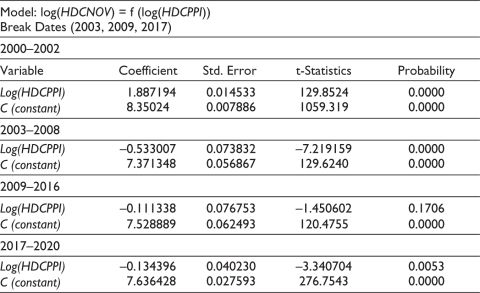
Table 7. Regression Model Coefficients for Paradip Port, with Number of Vessels (PARADIPNOV) = f(HDC (PARADIPPPI)).

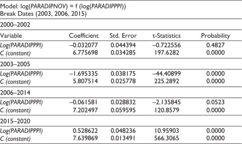
Source: EVIEWS 12 Student Version.

Table 8. Regression Model Coefficients for Visakhapatnam Port, with Number of Vessels (VISAKHANOV) = f(HDC (VISAKHAPPI)).

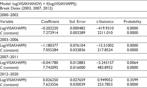
Source: EVIEWS 12 Student Version.

 

The test validity results are given by Table B1 to Table B3. Table 6 suggests that 2003, 2009 and 2017 are the structural breaks for the number of vessels (HDNOV) of HDC. Prior to 2003, between 2000 and 2002, the coefficient of Log (HDCPPI) was positive, indicating port performance impacted the number of vessels. In the following time segments, that is, 2003 to 2008, 2009 to 2016 and 2017 to 2020, the port performance (PPI) did no effect the number of vessels calling HDC. In the period 2009 to 2016, the coefficient was found to be insignificant at the 5% level.

The derived model in Table 7 suggests that in the period 2015 to 2020, the port performance significantly affected the number of vessels compared to the previous time segments when there was no positive effect.

Table 8 suggests that from 2012 to 2020, the port performance significantly affected the number of vessels compared to the previous time segments when there was no positive effect.

Managerial Implications

The results of the above analysis show that ports in India have inconsistent performance, and port reformatory measures did not impact performance uniformly across all ports. The success of reforms lay with the individual ports. Several ports had a reactive approach. This is illustrated by the findings as a drop in performance during a period is followed by improvement in the next. Ports that showed consistent performance can serve as a benchmark for their peers. The turnaround time of ships, dwell time of cargo and turn times of road carriers are crucial key performance indicators (KPIs) to monitor. These KPIs also lead to the derivation of sustainability of the ports. Higher waiting times, turnaround and dwell times lower the sustainability of the port as it refers to higher emission levels and energy consumption. Port performance can be improved through measures such as process improvements and capital investments in infrastructures (Sinha, 2011).

Ports may not always compete with each other, instead two ports can exhibit complementarity, that is, an increase in ship calls in a port also leads to an increase in the complementary port. The results of regression analysis show that poor performance did not affect significantly the performance of Haldia Dock Complex from 2009 to 2016. The ports of Paradip and Visakhapatnam, to some extent, also share common ship calls with HDC. This is because HDC has a low draft (around 8 meters) and cannot accommodate fully laden Panamax vessels (80,000 DWT). The fully laden ships that visit Paradip and Visakhapatnam partially unload cargo in these ports and carry the rest to HDC, depending on the demand but within the permissible navigable draft. The frequency of such visits makes HDC more dependent on the performance of the ports of Paradip and Visakhapatnam. This is the reason for the insignificant impact of PPI on the number of vessels calling at HDC.

Paradip and Visakhapatnam ports enjoyed monopolies prior to 2015 and 2012, respectively, as there were few competing ports. Port of Dhamra was built close (around 130 km) to Paradip port. It started its operation in 2011 and is now a competitor of Paradip port, as both setups handled the common dry bulk cargo. Visakhapatnam port now competes with minor (under state governments) ports of Krishnapatnam (set up in 2008) and Gangavaram (set up in 2009).

Thus, this study shows that ports can exhibit complementarity and competitiveness depending on the facilities and performance. Reforms had led privatisation of port services and the growth of private greenfield ports. These developments have led to increased competition. The ports in India are feeder ports (Kavirathna et al., 2021), depend on hinterland cargo demand and do not handle international transshipment cargo. Since there has been a proliferation of ports and terminals, one cannibalises the throughput of the other.

Conclusion

In the post-liberalisation period of rapid economic development, like other countries, India has also taken several reformations and port development measures to enhance operational efficiency and overall performance of its ports. Port researchers worldwide have already established that port performance positively affects port calls and productivity. Through this comprehensive study for the time period (1999 to 2020), we have tried to capture the true state of performance of the 13 major docks of India with a single composite performance index (PPI) for each port with respect to time. The SPPI for a port at a point in time shows time shows how it performs relative to its performance over time. PPI/SPPI shows that not all the ports are consistent with respect to performance, and the progress in performance enhancement is quite slow and varies significantly from port to port in spite of government initiatives for reformation through several programs in the last 15 years to enhance the performance of all the major ports.

The results of causality between port performance and ship call at a particular port showed varied outcomes. The effect of port performance on port calls varied from negative to positive and was sometimes insignificant in the case of the HDC and Visakhapatnam ports. The performance of the Paradip port for the last five years has had a significant positive effect on the port calls.

This article makes three crucial propositions—first, port performance affects its output, but the same may not impact the ship calls if the port enjoys monopoly or oligopoly status and due to other factors such as cargo demand. Second, performance of ports with lower capacity, also referred to as satellite ports, is affected by performance of its complementing ports with higher capacity. Third, reforms may lead to competition and cannibalisation of profits and growth of ports in a dynamic environment (Pancras et al., 2012).

As a future scope of work this analysis can be extended for all the ports and benchmarked against global ports. Besides, the extent of market concentration can also be studied over time.

Declaration of Conflicting Interests

The authors declared no potential conflicts of interest with respect to the research, authorship, and/or publication of this article.

Funding

The authors received no financial support for the research, authorship, and/or publication of this article.

ORCID iD

Deepankar Sinha https://orcid.org/0000-0001-9138-094X

Table A1. Descriptive Statistics for ATRT.

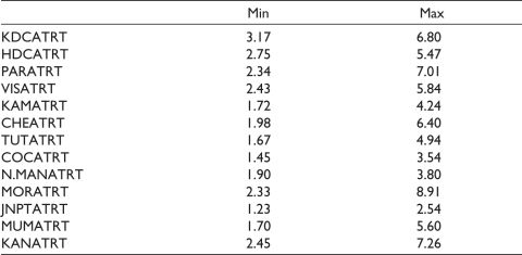
Source: Basic Port Statistics Report (2020–2021) of the Ministry of Shipping, Government of India.

Notes: KDCATRT: Average Turn Round Time of Kolkata Dock Comp; HDCATRT: Average Turn Round Time of Kolkata Dock; PARATRT: Average Turn Round Time of Paradip Port; VISATRT: Average Turn Round Time of Visakhapatnam Port; KAMATRT: Average Turn Round Time of Kamarajar Port; CHEATRT: Average Turn Round Time of Chennai Port; TUTATRT: Average Turn Round Time of Tuticorin Port; COCATRT: Average Turn Round Time of Cochin Port; N.MANATRT: Average Turn Round Time of New Mangalore Port; MORATRT: Average Turn Round Time of Marmagao Court; JNPTATRT: Average Turn Round Time of Jawaharlal Nehru Port; MUMATRT: Average Turn Round Time of Mumbai Port; KANATRT: Average Turn Round Time of Kandla Port.

Table A2. Descriptive Statistics for APBD.

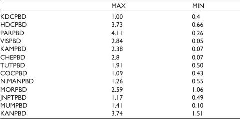
Source: Basic Port Statistics Report (2020–2021) of the Ministry of Shipping, Government of India.

Notes: KDCPBD: Pre-berthing Time of Kolkata Dock Complex; HDCPBD: Pre-berthing Time of Haldia Dock Complex; PARPBD: Pre-berthing Time of Paradip Port; VISPBD: Pre-berthing Time of Visakhapatnam Port; KAMPBD: Pre-berthing Time of Kamarajar Port; MUMPBD: Pre-berthing Time of Mumbai Port; CHEPBD: Pre-berthing Time of Chennai Port; TUTPBD: Pre-berthing Time of Tuticorin Port; COCPBD: Pre-berthing Time of Cochin Port; N.MANPBD: Pre-berthing Time of New Mangalore Port; MORPBD: Pre-berthing Time of Marmagao Court; JNPTPBD: Pre-berthing Time of Jawaharlal Nehru Port; KANPBD: Pre-berthing Time of Kandla Port.

Table A3. Descriptive Statistics for AOSBD.

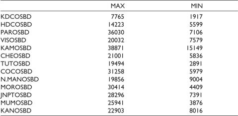
Source: Basic Port Statistics Report (2020–2021) of the Ministry of Shipping, Government of India.

Table A4. Descriptive Statistics for IT%.

 

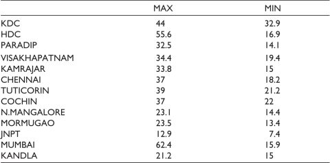
Table B1. Model Validity Test Statistics for log(HDCNOV) = f (log(HDCPPI)).

 

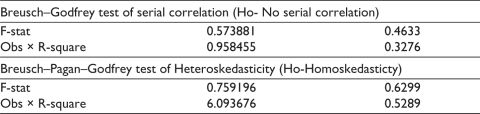
Table B2. Model Validity Test Statistics for log(PARADIPNOV) = f (log(PARADIPPPI)).

 

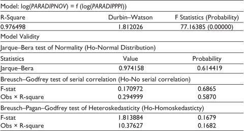
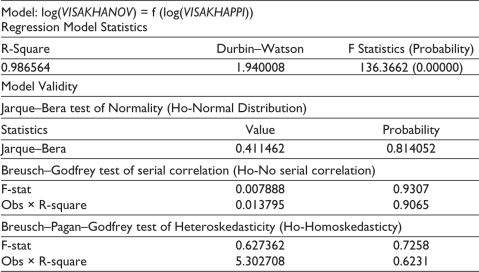
Table B3. Model Validity Test Statistics for log(VISAKHANOV) = f (log(VISAKHAPPI)).