Introduction

The exchange rate (ER) and interest rate (IR) dynamics occupy a central place in academic debates and policy framing. Any change in either of the two leads to massive changes in the macroeconomic outlook of the country concerned. While ER changes significantly impact the country’s net exports and imports, the IR changes lead to international capital flows and alterations in domestic investment and the overall economic scenario. ER changes constitute an important macroeconomic challenge for developing economies due to the fear of floating. Massive and destabilising ER fluctuations appear to be critical during times of economic crisis owing to huge associated costs and lengthy recovery processes.

Among several factors such as geopolitical risk, economic policy uncertainty, monetary and fiscal policy stances, the gyrations in the ER are also linked to IR changes. IR is among the many monetary policy instruments used to manage ER volatility. Specifically, raising the IR in a particular country appreciates its domestic currency in short run through capital inflows, however, coupled with an unfavourable effect on trade balance. In the long run, international investors would be required to convert the foreign currency-denominated investments and interest earnings into the local currency. As such, an increase in IR is likely to depreciate the ER in the long run.

The portfolio balance models (Branson, 1981; Branson & Halttunen, 1979; Branson et al., 1977) like the Mundell–Fleming model assert for an inverse relationship between IR and the ER, by assuming international capital mobility and price stickiness in the short run. On the contrary, in their incipient Redux model, Obstfeld and Rogoff (1995) anticipated the case of no expected appreciation or depreciation under uncovered IR parity. The monetary shocks merely result in a change in nominal IRs of the same magnitude in both nations, leaving the IR differential unchanged and hence no effect on ER. More recently, Betts and Devereux (2000) incorporated the pricing-to-market (PTM) strategy into their model using local currency pricing (LCP). The authors conclude that a monetary expansion under the PTM scenario would lead to a reduction of IR differential along with ER overshooting.

Despite the conflicting theoretical contours, it is widely admitted that tight monetary policy and higher IR can assist in stabilising ER fluctuations. Following the currency crisis, Goldfajn and Baig (1998) distinguished four building blocks for analysing monetary policy. First, determine whether the real ER has depreciated and has to be restored to its equilibrium level. Second, identify the relevant mechanism to adjust the real ER following any deprecation. Third, find suitable policies and circumstances that help in reverse through the appreciation. Finally, analyse the effects of increasing IRs. Expected gains from increasing IRs on the ER can be offset by increasing unemployment, output loss and financial system fragility.

 A plethora of studies, both theoretical and empirical, have been conducted in different economies using different data periods and econometric methodologies. Lily et al. (2011) used autoregressive conditional heteroscedasticity and generalised autoregressive conditional heteroscedasticity models and found that there is a substantial effect of uncovered IR changes on ER movements. Hacker et al. (2014) found that IR differential drives the ER volatility by using wavelet analysis and found a strong positive relationship in the long run and a strong negative linkage in the short run. Hnatkovska et al. (2013) examined a data set of 80 different economies in different regions, and have proven mathematically that there is a non-monotonic relationship between the IR and ER. However, Sollies and Wohar (2006) used symmetric and asymmetric approaches and found nonlinearity in IR and ER relationships. On the other hand, Abbas et al. (2012) and Saraç and Karagöz (2016) found no significant impact of IR on ER. From the previous literature, we can conclude that inconclusive evidence has been reported regarding the relationship between the IR and ER. The ER can move in any direction, and the IR can be used as a monitoring and controlling tool by the government.

 In this backdrop, this study attempts to examine the impact of IR changes on the ER fluctuations in case of five emerging market economies namely, Brazil, Russia, India, China and South Africa (BRICS). Studies regarding BRICS have been largely conducted in an individual country framework, and the BRICS as a panel has not been studied promptly. Moreover, the existing evidence is inconclusive and previous studies have ignored the inclusion of important determinants of ERs. We incorporated a panel linear ARDL model for our empirical exercise on the data spanning from Feb 1999 to August 2021. In addition to the fundamental determinants such as money supply growth rate, inflation and gross domestic product (GDP) growth, the responsiveness of ER has also been calculated with respect to two different IR measures for sensitivity analysis. Moreover, other relevant estimation methods have been incorporated for robustness purposes. The article contributes to the existing literature by providing comprehensive empirical evidence on the ER and IR nexus in the context of the BRICS countries. The results offer valuable insights for policymakers, central banks and market participants by shedding light on the intricate interactions between ERs and IRs. These findings can assist in formulating effective monetary policies, managing ER volatility and fostering economic stability in the BRICS economies.

The rest of the paper is organised as follows. The second section discusses the theoretical background. A brief summary of the recent empirical literature is given in the third section, the fourth section outlines the data description and econometric methodology, and the fifth section outlines data and descriptive statistics. Results are discussed in the sixth section, robustness check in the seventh section, and the eighth section concludes.

Theoretical Background

Theoretically, economic fundamentals determine the ER. One of the most important economic factors that impact the ER is the interest differential between domestic and foreign countries. Various economic models explain the nexus between IR and ER.

The portfolio balance models (Branson & Halttunen, 1979; Branson et at., 1977; Branson, 1981) suggested an inverse relationship between IR and the ER. Portfolio reallocations will be determined by the IR changes. When the domestic IR increases, a nation’s interest-bearing assets become more attractive, inducing investors to own more assets. This will lead to an appreciation of the domestic currency. The Mundell–Fleming model predicts an inverse relationship between IR and the ER, by assuming international capital mobility and price stickiness in the short run. In this situation, a lower IR in a domestic country causes capital outflow and a balance of payment deficit, which can be rectified by an increase in net exports through depreciation in the national currency.

Obstfeld and Rogoff’s (1995) in their Redux model, there is no expected appreciation or depreciation under uncovered IR parity. The monetary shocks will merely result in a change in nominal IRs of the same magnitude in both nations. Betts and Devereux (2000) significantly improved the model by incorporating PTM using LCP. They conclude that a monetary expansion under these conditions could reduce the IR differential along with ER overshooting.

On the other hand, we commence our analysis with two presumptions. The first assumption is Fisher’s (1930) hypothesis; this hypothesis states that an increase in a nation’s nominal IR ought to be proportional to any rise in the predicted level of inflation in that nation. The second is that the IR in one’s home country rises exogenously, not due to money market disturbances. The subsequent increase in price levels as a result of decreased demand for money may, therefore, result in an increase in the ER. Accordingly, Hacker` et al. (2012, 2014) mentioned that purchasing power parity theory (PPP) predicted a positive relationship between the IR and ER. This approach depends upon perfect price flexibility in the long run. The Keynesian approach also justifies the positive association between the IR and ER. The country’s trade balance improves as a result of an increase in the ER. This could lead to a rise in the country’s IR in the short term due to an increase in the aggregate demand for its products with sticky prices.

Dornbusch (1976) developed a model which is a combination of the two models that are complete opposites of one another. As a short-term characteristic, it consists of price stickiness in various product markets. However, the price adjustment over a long period towards its new equilibrium is one of the distinctive features of the flexible-price monetary model. Because of monetary shocks, the relationship between the IR and ER is inverse in the short run and are positively related in the long run.

Review of Literature

A plethora of studies have been conducted to examine the relationship between the ER and IR. Studies that examined the relationship between these two variables have found contradictory and/or mixed results. The differences appear due to which group of countries is analysed (emerging, developing or developed), which IR is considered (nominal or real IR; market-determined or policy controlled; short term or long maturity IR etc.), which type of ER regime is adopted.

Sanchez` (2008) has explored the relationship between the IR and ER in small open economy under flexible ER. He concluded that the IRs are raised in order to avoid the contractionary effects of currency depreciation in the face of an adverse risk premium shock. Furthermore, IRs are expected to rise in contractionary depreciation scenarios, while in expansionary depreciation circumstances, they are expected to fall. López and Raymond Bara (2008) have suggested an economic model for determining the real ER in Mexico, including long-run variables of the real IR, relative GDP per capita and the net foreign assets. In order to determine a dynamic adjustment in response to economic shock they used VAR model for impulse response functions. According to their analysis, the notion of PPP is flawed in the long run, and the real ER is linked to macroeconomic variables such as real IR, relative productivity and the stock of debt. While Tari and Abasiz (2009) argued that the causal relationship between the IR and ER is valid only for the short run. However, Uysal et al. (2008) identified a causal link between the IR and foreign ER.

Hnatkovska et al. (2013) investigate the nexus between the ER and IR and found that the relationship between them is non-monotonic. Furthermore, they found that the ER response relies on the preliminary level of IRs and the magnitude of the IR increase. Chin and Meredith (2004, 2005) found a positive association between IR differential and the log ER after using short and long maturity bond data. Utilising short-maturity bond data, they showed a negative correlation between these variables, but the results were the opposite when using long-term bond data. However, Flood and Taylor (1996) found a negative relationship when using short-term bond data, while they find a positive connection when they used medium-maturity bond data.

The study conducted by Vithessonthi (2014) in Thailand over the period 2003–2011, examined the link between the IR and ER showed that when the IR differential is high, an unexpected increase in the policy rate causes a major depreciation of Baht against the British pound and the US dollar. The researchers Granville and Mallicki (2010) believe that Russia’s monetary policy focuses more on ER stability than price stability, making IRs more sensitive to ER shocks. Kayhan et al. (2013) used nonlinear and frequency domain causality tests using monthly data of Brazil, Russia, India, China & Turkey (BRIC-T). Their analysis shows long-term IR implications on China’s ER. In contrast, only short-term changes in IRs can be noticed as a result of ER shocks. Using the frequency domain Granger causality test, Saraç and Karagöz (2016) investigated the connection between the IR and ER. They concluded that there was insufficient evidence to support the hypothesis that an increase in IRs would result in a reduction in the ER.

Ahmed and Mazlan (2021) used ARDL and NARDL models to study the effect of IR on ER across ASEAN economies. Their findings suggested that IR changes have a symmetric effect on ER in the short run and hold for five countries, namely, Malaysia, Cambodia, Singapore, Vietnam and Thailand, in the long run. However, IR changes have negative and asymmetric effects on ER for seven ASEAN economies, namely, Malaysia, Cambodia, Philippines, Singapore, Vietnam, Indonesia and Thailand, in the long run.

Issahaku et al. (2023) examined the relationship between the IR and ER in Ghana by using the monthly data spanning from 2007 to 2020. The results reveal a strong positive association between the variables. They also suggested that policymakers meticulously trace the IR and ER nexus to craft the policies for macroeconomic stability in the long run. Also, Demirhan and Göksu (2023) examined the relationship between ER and macroeconomic determinants in Turkey by using symmetric and asymmetric ARDL approaches. The main findings of the study are that there exists an asymmetric cointegration, but the relationship is not symmetrical among the set of chosen variables.

Analytical Framework and Econometric Methodology

We followed an analytical model proposed by Ahmed and Mazlan (2021) to examine the relationship between the dependent variable (ER) and other explanatory variables (IR, inflation, money supply and GDP). We extended their model by including GDP in the model as an additional explanatory variable because of relevant theoretical reasoning. The following model is used to scrutinise the possible impact of IR on ER changes along with inflation (INF), money supply growth (MSG) and GDP:

                                ??              

Accordingly, the estimable regression equation is specified as

                                (1)

where a0 is a constant term. a1, a2, a3 and a4 are the coefficients to be estimated, ‘t’ signifies the time and ‘?’ is the cross-sectional unit. ER, IR, INF, MSG and GDP are exchange rate, interest rate, inflation, money supply growth and gross domestic product, respectively.

Econometric Methodology

We assume the homogeneity of slope coefficients in Equation (1) would be unrealistic due to the heterogeneous nature of our panel. Instead, a dynamic heterogeneous panel model is needed. In the empirical literature, the Mean Group (MG) estimator and the Pooled Mean Group (PMG) estimator are the two popular approaches for analysing heterogeneous panels. The MG estimator involves the estimation of N time series regressions and averaging of the regression coefficients, whereas PMG employs the combination of pooling and averaging of coefficients (Blackburne & Frank, 2007).1 The variables must be I (1) and I (0) or a mixture of these two in order to use these methods, and the model must be cointegrated for the variables to be interpreted as an error-correction mechanism. Therefore, in the following part, we will first give the stationarity tests for the variables, followed by the existence of cointegration, and finally, the panel estimator using PMG estimation.

We start the examination of the relationship between ER and other explanatory variables using symmetric panel ARDL model, developed by Pesaran and Smith (1995) and Pesaran et al. (1999) by assuming symmetrical response of ER to changes in the various explanatory. The symmetric panel ARDL model is given as

                        (2)

where ER is the exchange rate for each economy ? over a period of time t. IR, INF, MSG, GDP are log of IR, inflation, money supply growth and gross domestic product, respectively. µi is the group-specific effects. β0i captures the country-specific effects, β1 is the AR coefficient,c2; c3; c4; c5 are long-run coefficients and β2; β3; β4 β5 are short-run coefficients. In the error-correction specification with ECT_{i, t – 1} as linear error-correction term for each country and di measuring the error-correction speed towards the long-run equilibrium following any short-run distortion, Equation (2) can be written as

                        (3)

For robust estimation to validate the results of panel linear autoregressive distributed lag (PARDL) estimation techniques like fully modified ordinary least square (FMOLS) and dynamic ordinary least square (DOLS) are used. The FMOLS regression technique was initially developed by Pedroni (2001), which is a residual-based test and delivers efficient results for variables that are cointegrated. In situations where the sample size is small, FMOLS is regarded as a reliable estimate and it eliminates the problem of serial correlation and endogeneity among the variables (Hamit-Haggar, 2012). However, DOLS was developed by Stock and Watson (1993). DOLS eliminates correlation among regressors and provides better results than FMOLS (Kao & Chaing, 2001). This study used both FMOLS and DOLS to confirm the consistency of the outcome. According to Hamit-Hagger (2012), the most suitable technique for panels with heterogeneous cointegration is FMOLS, which has the advantage of correcting serial correlation and endogeneity bias (Ozcan, 2013). The DOLS has the same asymptotic distribution as of FMOLS estimation derived by Pedroni (1996).

Data and Descriptive Statistics

The balanced panel includes observations of five emergent market economies, namely, Brazil, Russia, India, China and South Africa (BRICS), from 1999 (M02) to 2021 (M08).2 The data set contains six variables: call money rate (CMR) and Treasury bill rate (TBR) as a proxy for IR, ER defined as domestic currency per US dollar meaning that an increase in ER implies domestic currency depreciation, GDP, inflation (INF) and MSG. The data on CMR, TBR, GDP and MS are obtained from the Federal Reserve Bank of St. Louis (FRED). However, the data on ER and INF are obtained from the International Monetary Fund (IMF). Additional details pertaining to the data variables are reported in Table 1.

Table 1. Data Description.

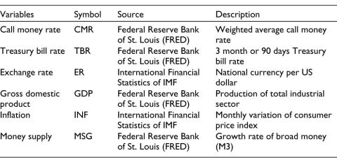
Note: Data with respect to broad money have also been obtained from DBIE of Reserve Bank of India and Central Bank of China. The data have been tested for seasonality using the parametric F test, the non-parametric Kruskal–Wallis test and the moving seasonality test. We de-seasonalised the data wherever required by applying the Census X13 algorithm of the Census Bureau of United States for a valid empirical exercise.

 

Descriptive Statistics

Table 2 summarises the descriptive statistics of monthly frequency data on ER, CMR, GDP, INF, MSG and TBR variables for the BRICS economies. The total number of observations across BRICS is 1,355. Table 1 confirms that the variable with the highest and lowest mean growth across BRICS is ER and GDP, respectively. The greatest variation as defined by standard deviation relative to mean is shown by ER across BRICS. We further find that the variables have only positive skewness in the distribution and excess kurtosis is positive for all the variables, meaning that the distribution is leptokurtic and the distribution is skewed more towards the right (positively skewed distribution).

Table 2. Descriptive Statistics.

 

Results and Discussion

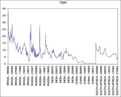
Our analysis starts by examining the time series plots of the variables (ER, CMR, GDP, INF MSG and TBR) as displayed in Figures 1–6. These figures help us understand the series’ visual properties such as trend, drift and structural breaks. Figure 1 illustrates the time-series plots of ER variables for all the BRICS economies. Similarly, other figures show the time plots of the rest of the variables across BRICS economies.

Figure 1. ER.

 

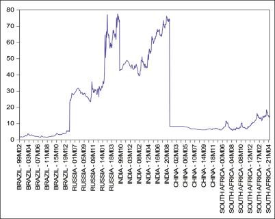
  Figure  2. CMR.

 

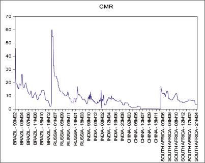
Figure 3. GDP.

 

Figure 4. INF.

 

Figure 5. MSG.

 

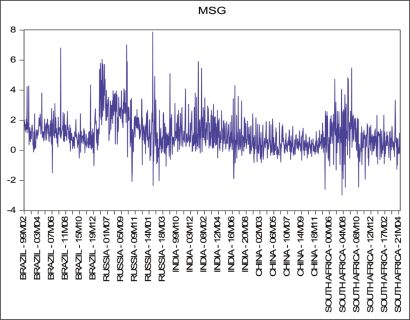
Figure 6. TBR.

 

Unit Root Analysis

We proceeded with the panel unit root testing to ascertain the stationarity properties. We applied several unit root tests like Levin et al. (2002)’s LLC test and Pesaran et al. (1997) LM test, wherein the former assumes homogeneity in the dynamics of AR coefficients for all panel members and the latter allows for heterogeneity. The non-parametric unit root tests of Maddala and Wu (1999) are also applied using Fisher ADF and Fisher PP tests. In all the cases, we test the null of non-stationarity against an alternative of a unit root. Results are reported in Table 3. We find a mixture of I (0) and I (1), and none variable is I (2), and, therefore, vindicate the application of a panel dynamic model.

Table 3. Unit Root Analysis.

Note: ‘a’ represents the stationary at level and ‘b’ indicates stationary at first difference respectively.

 

Panel Cointegration Test

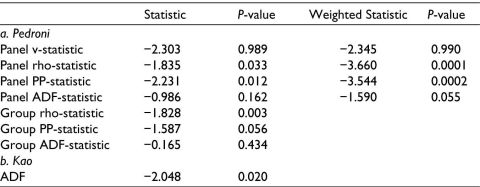
With a mix of I (0), and I (1) variables, we proceeded to check for the possibility of long-run cointegration among the variables. Pedroni’s (1999, 2004) residual-based heterogeneous panel cointegration test, which permits cross-section interdependence with distinct individual effects, is estimated. Since our BRICS panel is heterogeneous, using the Pedroni test is appropriate. To test the null of no cointegration, Pedroni (1999, 2004) developed 7 test statistics (Panel PP-statistic, Panel rho-statistic, Panel ADF-statistic, Panel v-statistic, Group PP-statistic, Group rho-statistic, Group ADF-statistic). All these test statistics are assumed to follow a normal distribution. To validate Pedroni’s (1999, 2004) results, Kao (1999) is also employed. Table 4 shows that out of seven Pedroni’s (1999, 2004) test statistics, cointegration is found in five tests when it is examined among (ER, CMR, GDP, INF and MSG). The test statistics reject the null of no cointegration and, therefore, establish the evidence in favour of a long-run association among ER, CMR, GDP, INF and MSG. Similarly, Table 5 reported evidence of cointegration in five out of seven test statistics, when examined among (ER, TBR, GDP, INF and MSG). The Kao tests in the lower panels of Table 4 and Table 5 again authenticate the presence of cointegration among the two sets of variables. Thus, it can be concluded that a long-run cointegration exists among the variables.

Table 4. Panel Cointegration Tests with CMR as Proxy for Interest Rate (LER, CMR, GDP, INF and MSG).

 

Table 5. Panel Cointegration Tests with TBR as Proxy for Interest Rate (LER, CMR, GDP, INF and MSG).

 

Empirical Results

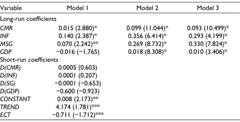
We begin with the estimation of model 1 (PARDL), model 2 (FMOLS) and model 3 (DOLS). Table 6 reports the results of all three models. In the long run, the impact of IR (CMR as a proxy for IR) is positive and statistically significant in all the models. This implies that an increase in the IR will cause depreciation of the ER across BRICS (or ER will increase). This phenomenon is due to the fact that an increase in domestic IR will lead to a fall in demand for money due to an expected increase in inflation and, hence, cause depreciation of domestic currency (Frankel, 1984; Sharma & Setia, 2015). Table 6 indicates that in the long run, a 1 unit increase in IR will increase the ER by 1.5%, 9.9% and 9.3% in models 1, 2 and 3, respectively.

Table 6. Results of ARDL, FMOLS and DOLS (CMR as a Proxy for Interest Rate).

Note: Figures in parentheses are t-statistic values. *, ** and *** indicate statistical significance at the 1%, 5% and 10% levels, respectively.

 

 On the other hand, the effect of money supply and inflation on the ER, in the long run, is positive and statistically significant, implying that an increase in money supply and inflation will cause domestic currency depreciation. This happens because an increase in money supply will cause an increase in the purchasing power, hence demand-pull inflation, thereby leading to a decrease in exports (higher inflation creates lower demand for exports) and thereby currency depreciation.

Lastly, the impact of GDP is positive and statistically significant in models 2 and 3 but is insignificant in model 1. This implies that an increase in GDP will increase the ER (currency depreciation). This is because an increase in GDP will increase imports more than exports, hence, capital outflow and, therefore, currency depreciation.

 On a comparative note, the impact of inflation on the ER fluctuations is substantial as followed by MSG, GDP and CMR, respectively. Finally, regarding the error-correction coefficient, the negative sign establishes the indirect evidence of long-run association. Model 1 reported a speed of correction of 0.711, suggesting that disequilibrium would be corrected by 71.1% per month.

Robustness Check

To check the reliability of the coefficients, we estimated an additional model with TBR as a proxy for IR. The results are in line with the above models. Table 7 reported that IR has a positive and significant effect on the ER in all models. Similarly, an increase in INF and MSG will cause ER to increase (currency depreciation). Lastly, the impact of GDP is positive and statistically significant in models 2 and 3 but insignificant in model 1 (see Table 7). This implies that an increase in GDP will depreciate the domestic currency. Again, the inflation is found to be dominant determinant of ER fluctuations as compared to other explanatory variables incorporated into the analysis. The error-correction term is again negative and significant, implying that equilibrium will be corrected by 81.1% per month.

Table 7. Results of ARDL, FMOLS and DOLS (TBR as a Proxy for Interest Rate).

Note: Figures in parentheses are t-statistic values. *, ** and *** indicate statistical significance at the 1%, 5% and 10% levels, respectively.

 

Conclusion

The IR and ER nexus has long been a focus of researchers and policymakers. This study attempts to examine the impact of IR on ER in the case of the world’s five emerging market economies, namely, Brazil, Russia, India, China and South Africa (BRICS), using the monthly data from 1999 (M02) to 2021 (M08). For the empirical exercise, the PARDL model developed by Shin et al. (2014), FMOLS developed by Pedroni (2001) and DOLS developed by Stock and Watson (1993) were incorporated to ensure the relationship among the variables. In addition to IR, the possible impact of inflation, money supply and GDP is also estimated. Incorporating the monthly data from 1999 (M02) to 2021 (M08) the results suggested that IR impacts ER positively, meaning that an increase in IR will increase ER (increase in ER implies currency depreciation). However, the impact of all other explanatory variables is also positive and statistically significant in the long run.

Policy Implications

The findings of this article lead to some important policy implications. It shows that an increase in IR attracts more foreign capital flows, increasing the demand for domestic currency and ER appreciation, which affects the country’s net exports and imports (trade balance), domestic investment and overall macroeconomic scenario. Thus, monitoring the IR and ER becomes crucial for the efficiency of monetary policy.

Declaration of Conflicting Interests

The authors declared no potential conflicts of interest with respect to the research, authorship and/or publication of this article.

Funding

The authors received no financial support for the research, authorship and/or publication of this article.

ORCID iD

Aijaz Ahmad Bhat  https://orcid.org/0000-0001-9835-5691

Notes

1. More specifically, MG assumes that intercepts, slope coefficients (both short-run and long-run) and error variances are allowed to vary across panel members. On the other hand, PMG estimator allows intercepts, error variances and short-run coefficients to vary, whereas the long-run coefficients are assumed to be uniform.
2. The choice of data period is made based on data availability.